Gorka Zamora-López

Analysing and interpreting data can be a complicated procedure, a maze made of interlinked steps and traps. There are no official procedures for how one should analyse a network. As it happens in many scientific fields the “standard” approach consists of a set of habits that have been popularised in the literature – repeated over-and-over again – without always being clear why we analyse networks the way we do.

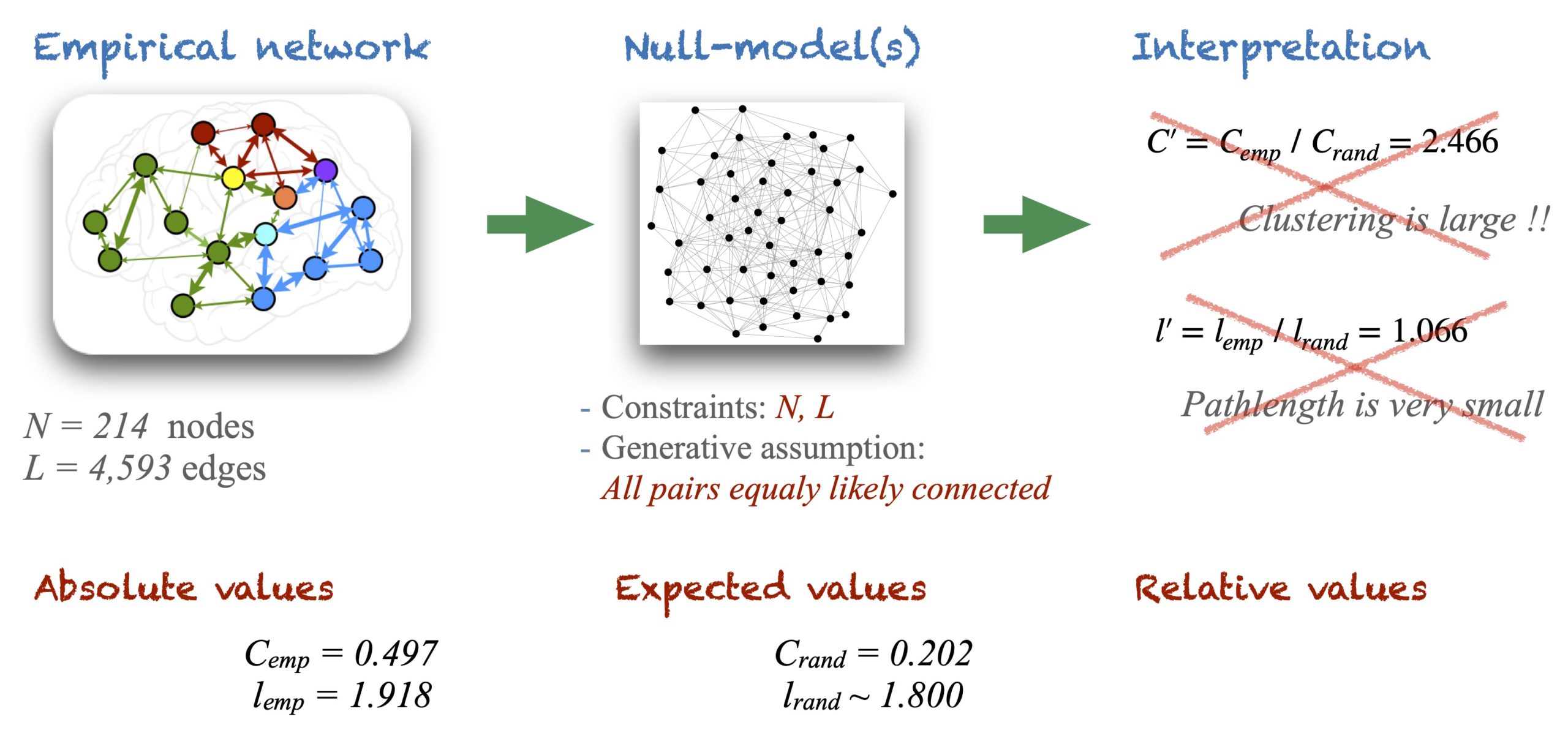
Imagine we wanted to study an anatomical brain connectivity made of \(N = 214\) cortical regions (nodes) interconnected by \(L = 4,593\) white matter fibers (a density of \(\rho = 0.201\)). Following the typical workflow in the literature we would start the analysis by measuring a few basic graph metrics such as the degree of each node \(k_i\) and their distribution \(P(k_i)\), the custering coefficient \(C\) and the average pathlength \(l\) of the network. Imagine we obtain the empirical values \(C_{emp} = 0.497\) for the clustering and \(l_{emp} = 1.918\) for the average pathlength.

The typical workflow would then lead us to claim that network properties depend very much on the size and the number of links and therefore, the results need to be evaluated in comparison to equivalent random graphs, or to degree-preserving random graphs. At this point, we would generate a set of random graphs of same \(N\) and \(L\) as the anatomical connectome, and we would calculate the (ensemble) average values \(C_{rand} = 0.202\) and \(l_{rand} = 1.800\). Finally, we would conclude that since \(C’ = C_{emp} \,/\,C_{rand} = 2.466\) our connectome has a large clustering coefficient and, since \(l’ = l_{emp} \,/\, l_{rand} = 1.066\) the connectome has a very short pathlength. Therefore, it is a small-world network.

Unfortunately, this line of reasoning is misleading because it skips some intermediate steps that are necessary for an adequate interpretation of the results.

Relative metrics are not absolute metrics

Let me expose this problem through a fictional example. Imagine that an old woman goes to the doctor’s and the doctor says: “I have good news and bad news for you. Unfortunately, the recent test shows you have 90% chance to develop lung cancer. The good news are, since you have been a heavy smoker for the last thirty years, there is nothing abnormal about it. So, go home and continue with your life as usual.”

The doctor’s recommendation is obviously absurd. Why? Because in that room, in that moment, the crucial information is that in a scale from 0 to 100% the patient is very close to developing a fatal disease. What matters in that scenario is to first answer the question “is the patient at risk of developing a cancer“? That information alone (90% chance) is sufficiently relevant to cause a strong reaction by the doctor and the patient, who will need to alter her lifestyle. Whether the result of the clinical test is expected or not as compared to some hypothesis – e.g. because of her age, because the woman is a heavy smoker, because she worked twenty years in a chemical factory or because of some genetic factor – that is rather irrelevant for the inmediate decision-making. Those other questions could be of importance, however, for a scientist investigating what are the causes of lung cancer, or to a lawyer considering whether they shall sue a tabaco company or the chemical factory in which the woman used to work.

This imaginary story exposes two of the matters that often go down the hill when analysing data and interpreting the outcomes:

1. Only because an observation is expected that doesn’t imply the observation is irrelevant. Neither does the other way around: that an observation is unexpected or significant doesn’t always mean it is relevant.
2. Null-models – used to calculate those expectations – are to be considered only when, and only where, they are needed.

In this case, the observation (the absolute or the empirical value) is that the test returns a probability \(P_{obs}(x) = 0.90\) for the patient to develop lung cancer. Apart from that, the doctors may have wanted to contrast the result with some factors, e.g. the age (a) of the patient and the number of years (y) she has been smoking. The parameters \(a\) and \(y\) are constraints which, introduced into a null-model, could have returned an expected probability of \(P_{exp}(x | a,y) = 0.87\). Finally, the doctor reads the relative value \(P’ = P_{obs} \,/\, P_{exp} = 1.03\) and since this is very small, concludes that the patient doesn’t have a problem. The absurdity of the case is that – same as it has been popularised for network analyses – the doctor reads the relative metric \(P’\) to provide an interpretation about the magnitude of the observation \(P_{obs}(x)\).

We shall keep in mind that absolute values are meant to answer questions about the magnitude of an observation such as “is the clustering of a network large?“, “is the pathlength of a network short or long?“, “is probability \(P(x)\) large or small?” On the other hand, relative values are only useful to answer comparative questions like “how similar is A to B” or “how does A deviate from B?” In order to judge whether the clustering of a network is large or small, we need to judge the empirical value \(C_{emp}\). Interpreting \(C’ = C_{emp} \,/\, C_{rand}\) instead for that purpose is misleading because we are demanding the relative value \(C’\) to answer a question it cannot answer. For the same reason that \(P’ = P_{obs}(x) \,/\, P_{exp}(x|a,y)\) is not an answer to whether the patient has a large or a small probability of developing a cancer.

Null-models are built upon two types of ingredients: constraints and generative assumptions. In random graphs the conserved numbers of nodes \(N\) and links \(L\) are the constraints. The generative assumption is that during the construction of the network links are added considering that any pair of nodes is equally likely to be connected. The values \(C_{rand}\) and \(l_{rand}\) are expectation values out of the null-model because their outcome depends both on the constraints and on the hypotheses we made of how the null-model is generated. Therefore, the relative metrics \(C’ = C_{emp} \,/\, C_{rand}\) and \(l’ = l_{emp} \,/\, l_{rand}\) are only meant to investigate whether \(C_{emp}\) and \(l_{emp}\) may have originated following the assumptions behind the null-model, not to evaluate how large / small or how relevant / irrelevant \(C_{emp}\) and \(l_{emp}\) are.

So, how to fix this?

The reason we analyse data is because we have some question(s) about the system we are investigating. To analyse data is thus to ask those questions to the data in the form of metrics and comparative analyses. Every metric we measure serves to answer a specific question. Every comparison we make as well. Besides, analysing data is a step-wise process that requires to follow a reasonable order. In my experience I came to realise that most incongurencies in the interpretation of data – including  some of the most heated debates – occur when we try to answer the wrong question at the wrong step, or when we evaluate the wrong metric for the question we aim at answering. Therefore, we need to be more aware of the steps we take to study networks and which are the questions we are targeting at each step, with every metric.

When a new network falls in our hands, one we have never seen before, our first goal is to understand “how does that network look like.” To answer this we don’t need null-models. At this initial step our job is to apply a variety of graph metrics available, to evaluate their relevance individually and together, such that the “picture” of the network takes form and makes sense. Once we have clarified the main properties of the network and its architecture, only then, we shall move onto the second step and start asking higher level questions such as “where does the clustering coefficient of this network come from?” Or, “why does this network have a rich-club?” Or, “how does this network compare to others of similar kind?” Answering those questions requires testing different hypotheses, posed in the form of generative assumptions on how the network may have arised. We will then build null-models based on those hypotheses and we will compare their outcomes (the expectation values) to the observations in the empirical network. This comparative exploration helps us determine whether our generative assumptions could be right or wrong.

Boundaries and limits, the forgotten members of the family

In summary, analysing a network implies two major steps. The first is to discover the properties and the shape of the network. The second step consists of inquiring where do those properties come from. For the latter, we will perform comparative analyses against null-models or against other networks. But, how do I to properly read the relevance of graph metrics in the first step, if it is not by comparing to other networks?

Well defined metrics have clear boundaries and those boundaries correspond to unambiguous, identifiable cases. For exampke, the Pearson correlation takes values from 0 to 1; \(R(X,Y) = 0\) when the two variables are (linearly) unrelated and \(R(X,Y) = 1\) only when the two variables are perfectly related (linearly). Those two boundaries, 0 and 1, and their meanings are the landmarks we need to interpret whether any two variables are correlated or not. If I were studying two variables and find that \(R(X,Y) = 0.21\), then I would know that \(X\) and \(Y\) are not correlated. To derive this conclusion it doesn’t matter what a null-model returns as an expectation under some given assumptions or how does this result compare to other cases. What matters is that, in a scale of 0 to 1, \(R(X,Y) = 0.21\) is very close to the lower bound.

In networks, many metrics have well-defined upper and lower boundaries as well. For example, a node could minimally have no neighbours and thus its \(k_i = 0\); or maximally, it could be connected to all other nodes such that \(k_i = N-1\). In the case of the average pathlength, the smallest value it can take is \(l = 1\), if the network is a complete graph. The longest possible (connected) graph is a path graph, whose average pathlength is \(l = \frac{1}{3}(N+1)\). The pathlength of disconnected networks is infinite but their global efficiency can be calculated. Global efficiency is minimal, \(E = 0\), in the case of an empty graph (a network with no links) and it is maximal, \(E = 1\), for complete graphs. These boundaries and their corresponding graphical configurations are the natural landmarks that help us evaluate whether a network has a short pathlength (large efficiency) or long (small efficiency).

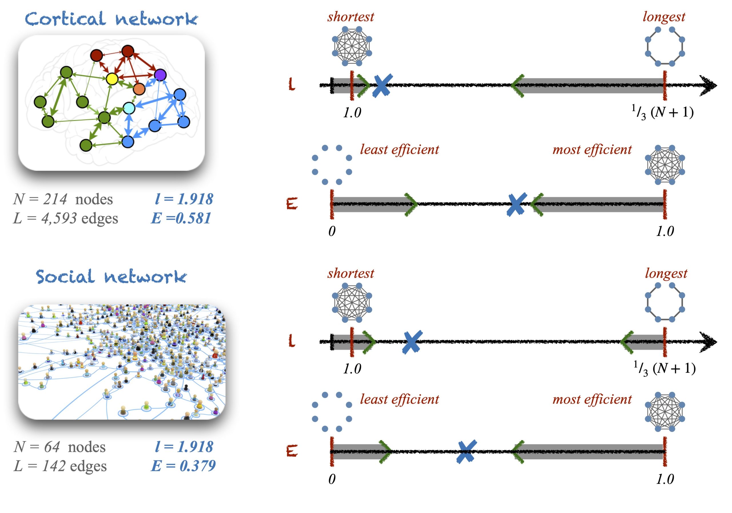
Now, we also have to acknowledge that, in occasions, the upper and the lower bounds could represent impractical solutions. For example, I just mentioned that the boundaries for the pathlength and for the global efficiency are characterised by empty graphs, complete graphs and path graphs. These configurations can only happen for specific combinations of \(N\) and \(L\) so, what happens with networks of arbitrary size and density? In those cases, there is no need to invoke null-models for help. Instead, what we really need is to identify the limits of the pathlength and efficiency for given \(N\) and \(L\), and use those limits in combination with the boundaries as references to  make the judgements.

Identifying the practical limits for all network metrics can be a difficult challenge but it is a necessary effort the community should face. In Zamora-López & Brasselet (2019) we could identify the upper and the lower limits of the average pathlength and of the global efficiency for (di)graphs of any arbitrary combination of \(N\) and \(L\). Barmpoutis and Murray (2011) accomplished the same for the betweeness centrality, the radius and the diameter of graphs. I am sure that completing the list of graph metrics with known analytical limits will help the field to achieve more transparent and more accurate interpretations, and will help restrict the use of null-models for those situations and questions for which they are truly helpful.

Concluding …

I have tried to expose why the popular workflows to analysing networks overstates the use of null-models. I hope the following take-home messages became clear:

1. Data analysis is all about asking questions to the data. Every network metric (absolute, expectation or relative) serves the purpose to answer a given but different question.
2. Analysing a network is a step-wise process and every step is also meant to answer different types of questions. First, we want to understand how the network looks like and second, where does its architecture come from or how it compares to other networks.
3. Null-models are an important tool for the questions in the second step because they are built based on constraints and generative hypotheses. Null-models are thus meant for hypothesis testing, not for assessing the magnitude of an observation.
4. Relative metrics such as \(C’ = C_{emp} \,/\, C_{rand}\) do not inform whether \(C_{emp}\) is large or small. For that, the boundaries and the practical limits of the metrics need to be considered as the landmarks that allow us to judge the magnitude (and the importance) of \(C_{emp}\).

For brevity I had to leave many matters aside in this post. Specially important are the practical implications for how to classify hubs, how to identify rich-clubs without relying on null-models, when is a network small-world and what are the consequences for community detection. Indeed, I would dare to say that the systematic use of null-models for community detection methods, e.g., via diverse modularity measures, biases their results. I hope to treat those topics in future posts.

So far, feel free to leave your views and comments below. And, if you would like to write your own post, let me know 🙂 Please notice that comments will be moderated and therefore they won’t appear inmediately. Comments should accept mathematical equations using LaTeX notation.

References

D. Barmpoutis & R.M. Murray “Extremal Properties of Complex Networks.” arXiv 1104.5532 (2011).
G. Zamora-López & R. Brasselet “Sizing Complex Networks.” Comms. Phys. 2:144 (2019).

---

About the Author(s)

Gorka Zamora-López is a post-doctoral researcher with +15 years of experience in the field. Now, he replies e-mails, attends zoom meetings and makes colourful figures all day long.